
(if you want to see code – check part II)
Since this is my first post, I thought I’d start with something I could not find anywhere on the net – an algorithm for taking gridded data (for example, in GRIB format), and turn it into contour line vectors.
I needed this type of algorithm when I wanted to add a meteorological layer to our GIS application. After some digging, I found some data sources I could use to get current wind speed and direction, waves height, and barometric data.
The custom way to display barometric data on a map is using Isobar vectors. Unfortunately, the data I found was a grid of data – a sample value every 0.5 degree, starting from the top-left corner of the area of interest.
I couldn’t find an answer on how to project this gridded data into isobar vectors, although commercial applications claim to do it.
Then I remembered that when I was in the navy, and we needed to get a meteorological report at sea, I saw how the meteorology guy plotted the data he got on a page, and then continued to mark grid-lines between plots, to later create vectors from them.
Since this was almost 15 years ago, and I didn’t really care then what he did, this was all I had to go on – and this is what I came up with:
Step I – set your values on the grid
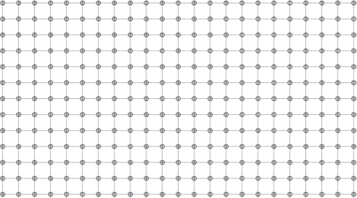 |
| A grid with values |
For the sake of simplicity, it is assumed that the starting point of the grid is at coordinates (0,0) (that’s Greenwich), and the distance between samples is 1x in every direction. Of course, the results can be scaled and translated to any other starting point/distance.
Step II – find adjacent points whose values cross over threshold levels
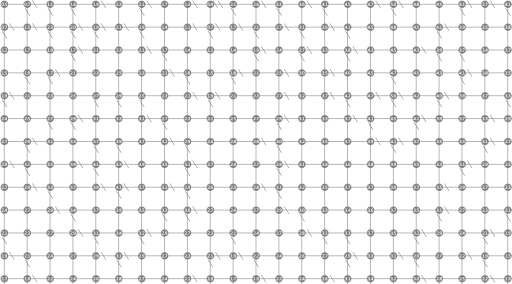 |
| Grid lines where threshold is crossed are marked |
Go over all the points on your grid, whenever a threshold (in our example – a whole number) is passed (either vertically or horizontally) – mark the grid line.
Gotcha – a threshold may be passed more than once between two adjacent points – see the first line in the example above – there is a jump from 0.9 to 2.1…
Step III – set threshold points, giving them location and direction
 |
| Contour points with location and direction |
Location heuristic is very naive – we presume that between two measurement points the graph is linear.
For direction the rule says – you circle a mountain clockwise. This means – if the high point is to my east – I’m going north; if it is on my north – I’m going west, and so on.
Step IV – connect the dots
 |
| Grid with isobars |
Here we use a few mathematical lemmas:
1) For every arrow entering a cell (which is not already used in an isobar) there must be at least one arrow with the same value exiting the cell which is not already used in an isobar.
2) Every isobar starting at the rim of the grid is open (not a circle).
3) All other isobars (which do not start at the rim) are closed.
With those lemmas, the algorithm is quite simple:
1) Go along the rim of the grid, and wherever you find an arrow entering the grid (south bound on the north rim, east bound on the west rim, etc.) follow it to create an open isobar.
2) Go over the inner points, and look for arrows which do not participate in any of the previous isobars. Follow each of those to create the closed isobars.
Following an arrow means – take the arrow and follow an arrow with same value which exits the cell the former arrow has entered. Stop when either you reached the rim or you encountered an arrow which is already selected for this isobar.
That’s it!
A word about edge cases
Besides the edge case already mentioned above, where between two grid points there is more than one threshold passed, there are two other edge cases worth mentioning:
Grid point is on the threshold – when a grid point itself is exactly on a threshold is potentially an edge case. To prevent this, I initially thought I’d avoid it altogether by adding an ‘epsilon’ amount to the grid point (which should not matter, as these should be real world values, which have measurement errors anyway).
As it happens, grid points with whole values worked perfectly without this workaround, and threshold points were marked as expected in this case as well.
More than one arrow with same value exiting a cell – sharp-eyed readers may have noticed that lemma number (1) hints on an interesting case – when there is more than one arrow with same value exiting a cell. This case happens in the following scenario:

 |
| Solution I |
 |
| Solution II |

One thought on “Creating Isolines (Contours) from grid data – part I”